ggplot: Aesthetics

The Robey dataset

In order to explore this topic thoroughly, we will be using R and a dataset called Robey that is already preloaded into R Studio. The dataset contains information about total fertility rate and contraception usage amongst developing countries from 1992. For more information, type in ?carData::Robey in your console. To access the dataset, we need to load it into our workspace. We do this, by assigning the dataset to a variable, e.g. Fert_Contra. 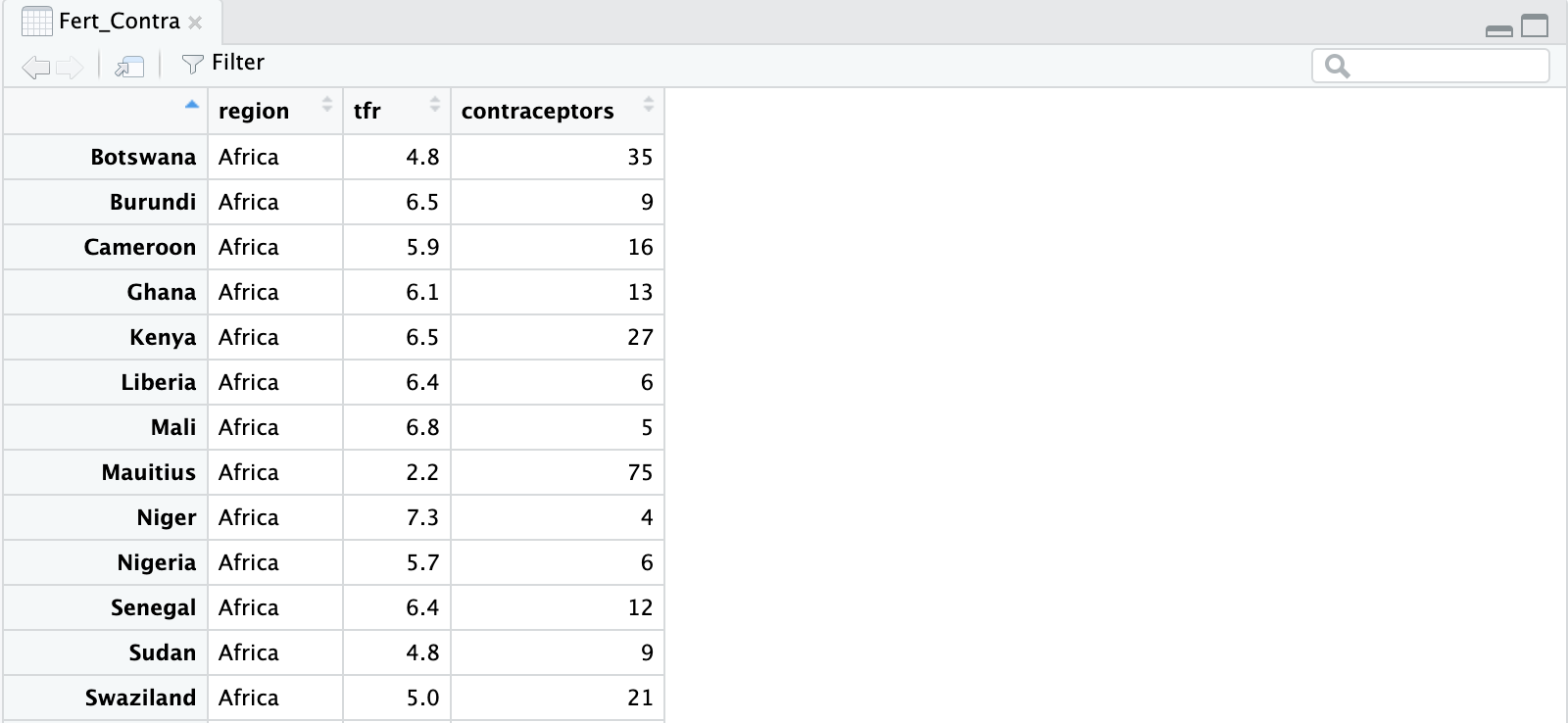Using the View function, we can look at the data in a new window:

# load the dataset into your workspace
Fert_Contra <- data(carData::Robey)

# get an overview of your data using the View function
View(Fert_Contra)

The View function will show the dataset in a table format as seen below:

note

You also need to load the ggplot package into your workspace before you can use it. To do so, type library(ggplot2) into the console.

What are aesthetics?

Aesthetics are used to map different information to certain visual properties in a plot. Mapping means that a variable from the specified dataset is linked to the plot in R to display it accurately. Examples of aesthetics include the size, colour or shape of the points in a plot. The mapping of variables to the x- or y-axis are also aesthetics.

You apply the aesthetic function by using aes() after typing ggplot2. Consider the following:

# create a scatter plot displaying the relationship between the total fertility rate 
ggplot(Fert_Contra, aes(x = tfr, y = contraceptors)) + geom_point()

This example of code contains the three essential parts that are always needed to create a graph in ggplot2:

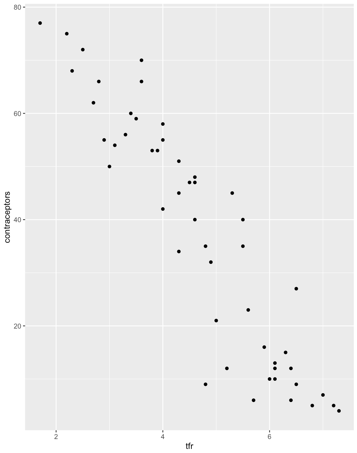
• ggplot(): the coordinate system that you add layers to. The Fert_Contra argument is the dataset that you want to visualize.
• aes(x = tfr, y = contraceptors): The aesthetics argument, that maps the variables to the x and y axes of the plot.
• + geom_point(): adds a geometry layer to your plot. This particular geometry function adds a layer of points so that a scatter plot is created. There are different geometry functions that create different plots (which will be explained in the next chapter).

The resulting plot will look like this:

You will usually have more variables in your dataset that you may want to display on a single plot. You can display more variables in one plot by mapping them to additional aesthetics such as colour and size.

Colour Aesthetics

To use this aesthetic add colour = inside the aes() function:

# create a plot that shows the relationship between tfr and contraceptors amongst different regions 
ggplot(Fert_Contra, aes(x= tfr, y = contraceptors, colour = region)) 
    + geom_point()

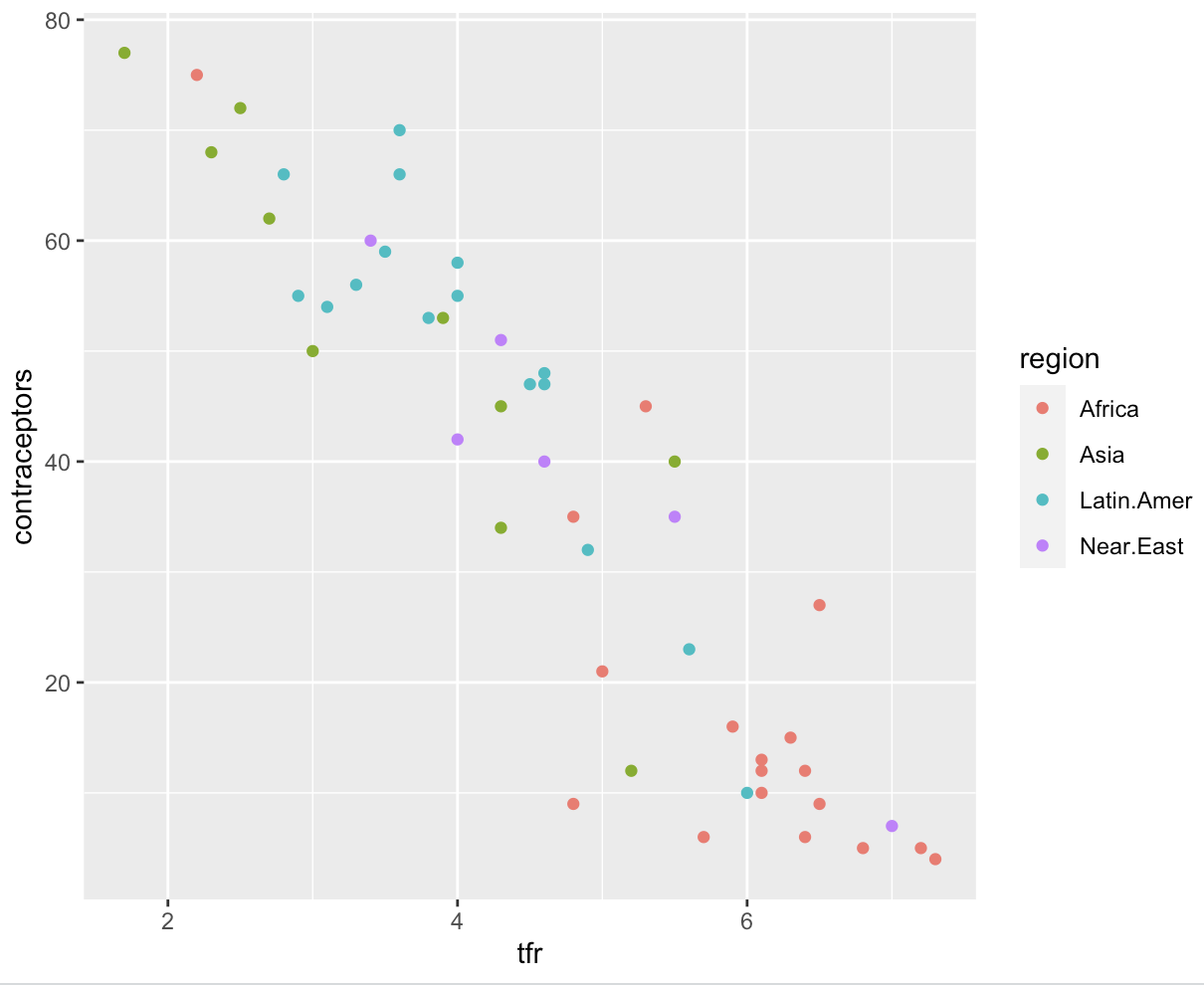
In the above code we added an argument in the aes() function in which the region variable was mapped to the colour aesthetics. This assigns a unique colour to each value in the variable. ggplot2 automatically adds a legend to the plot to show which values correspond to which colours:

Size Aesthetics

If you have a variable with numerical data, you can use size. To use this aesthetic, you add size = inside the aes() function:

# create a plot that shows the relationship between tfr and contraceptors amongst different regions 
ggplot(Fert_Contra, aes(x= tfr, y = contraceptors, size = region)) + geom_point()

In this example, region was mapped to the size aesthetic, where the size of each point corresponds to a certain region. However, since mapping a categorical data with the size aesthetic is not recommended, R will send out a warning along the lines of "Using size for a discrete variable is not advised":

note

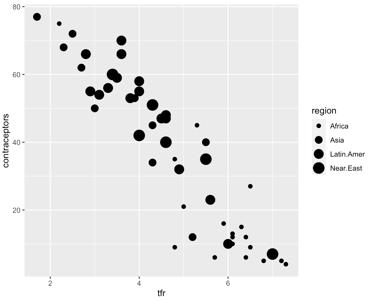
The greater the size of the dots, the larger the value the dot represents!

Alpha Aesthetics

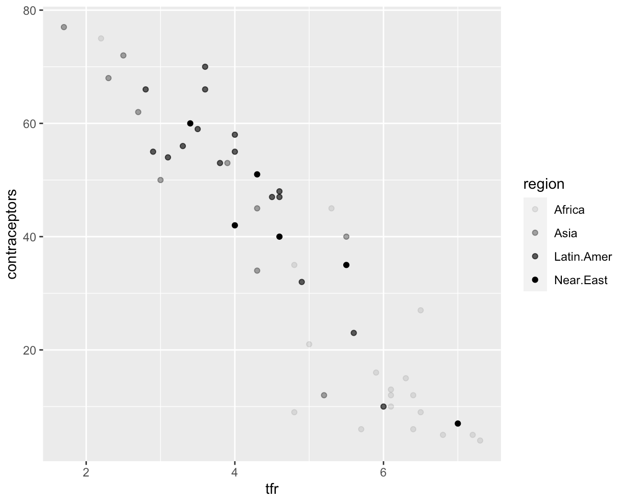
Using the alpha argument you can alter the transparency of your points:

# create a plot that shows the relationship between tfr and contraceptors amongst different regions 
ggplot(Fert_Contra, aes(x= tfr, y = contraceptors, alpha = region)) + geom_point()

In this case, region was mapped to the alpha aesthetic, with the transparency corresponding with a region. There will also be a warning message since we are mapping a categorical data with an aesthetic that is better used for numerical data:

info

The alpha argument can also be used to change the transparency of all points in a plot to the same value. The default value for alpha is 1. To reduce the transparency, you can set alpha to a value less than 1 (and larger than 0), outside aes() and inside the geom layer:

ggplot(Fert_Contra, aes(x= tfr, y = contraceptors)) + geom_point(alpha = 0.7)

Which gives the following result:

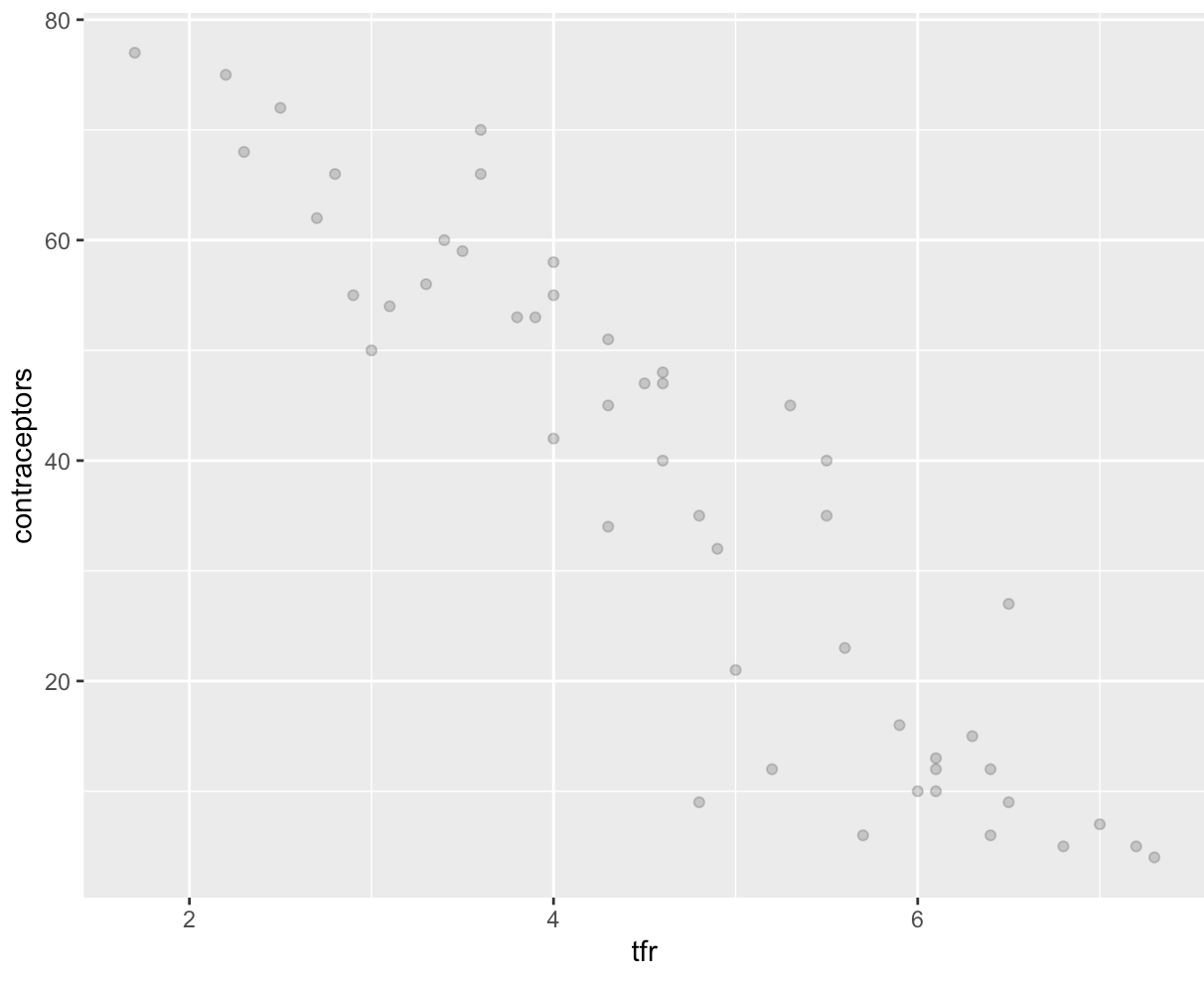
This syntax is usually used in an attempt to solve the problem of overplotting; in large datasets the dots are often all over each other and cannot be distinguished!

Shape Aesthetics

Categorical variables can also be mapped onto a plot using the shape aesthetic:

# create a plot that shows the relationship between tfr and contraceptors amongst different regions 
ggplot(Fert_Contra, aes(x= tfr, y = contraceptors, shape = region)) + geom_point()

This will translate into the following plot:

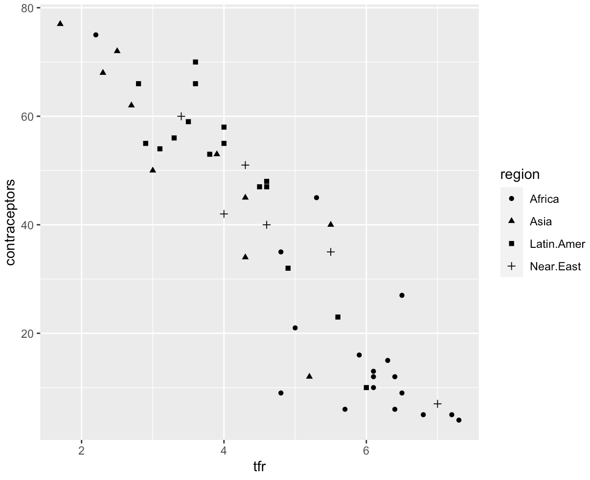
ggplot2 has 25 different shapes to choose from. The shapes seem to repeat themselves, but there are differences in their properties:

• Shapes 0 to 14 can only change the colour of their outline using the colour argument.
• Shapes 15 to 18 are filled with colour.
• Shapes 21 to 24 have an outline which can be modified using colour and the insides can be modified using fill.

Common aesthetics summary

The table below shows a summary of many aesthetics that are used to map information to a plot:

Aesthetic:	What it does:
x	maps variables to the x-axis
y	maps variables to the y-axis
colour	maps variables (preferably categorical) to outline colour
fill	maps variables (preferably categorical) to fill colour
shape	maps variables (preferably categorical) to shape
size	maps variables (preferably numerical) to size
alpha	maps variables (preferably numerical) to transparency
line type	maps variables to line type
labels	maps variables to certain words.