Automated 3D MRI Segmentation with nnU-Net
In this tutorial we learned how to segment a 3D MRI image with 3D Slicer. There, we had to set the segment seeds by ourselves before the software could calculate the segments. Another method, which doesn't require as much human input, is utilizing deep neural networks. In the following, we will use the pretrained deep learning model nnU-Net for automated image segmentation on our 3D MRI images. Be aware, that we not only will use Python code but also bash commands (Linux shell). Furthermore, we will execute the whole programm in Google Colab because it requires more computing power than our computers probably have.
Working with Google Colab
To use Google Colab, visit this website and log in with your Google account. Then, create a new Jupyter notebook by hitting "File" in the toolbar and selecting "New notebook".
We want to use a GPU for executing our program. To do this, click on "Additional connection options" as shown below (red box):
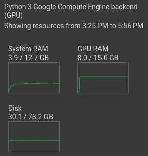
Select "Change runtime type". Then tick "T4 GPU" and save. Now, the GPU should be shown under "resources":

Install required packages
Now, we can start with our code. First, we need to install the required Python packages, on which nnU-Net depends. Because nnU-Net uses the PyTorch library, we need to install it first, before we install the nnU-Net package. Create a new code cell as shown in the graphic below.
Now, execute the following commands. Pay attention, that you don't change the order. The ! at the beginning of the lines are needed because these are bash commands and we want to use them in our Jupyter notebook.
!pip install torch
!pip install nnunetv2
Probably, there will appear a warning after installing nnU-Net, that you should restart the runtime, but you don't have to do that.
Set up datasets
For working with Google Colab, the following steps have to be taken while being in Google Drive, so the data can be accessed in Colab.
Never upload non-anonymized patient data to a cloud.
Directory structure
A special directory structure is required for nnU-Net to be able to access the data. First, create a new directory in Google Drive, in which you want to save your datasets. Now in this directory, create three more folders with the following names:
- nnUNet_raw
- nnUNet_preprocessed
- nnUNet_results
We can save new datasets in the "nnUNet_raw" directory. Every dataset has to have a specific name. It always starts with "Dataset", is followed by a three digit integer, which is the dataset ID, and ends with a description. In the following graphic you can see some examples.
The ID and the description can be chosen by the user, but the ID should not collide with already existing ones, which you can find here.
The last thing we have to consider, regarding the directory structure, is that every dataset folder has to include the following directories:
- imagesTr
- labelsTr
The "imagesTr" directory will include the training images and the "labelsTr" directory the corresponding segmentation files. You can also create a "imagesTs" folder, where you can save test images, but it is is not necessarily required for running nnU-Net.
Adjust the file format
Our data needs to be transformed into a usable form for nnU-Net. nnU-Net supports different file formats. In this case we will use NRRD files. The associated segmentations to the MRI images need to be exported as labelmaps. For this, we will use 3D Slicer again.
First, open your DICOM file with the corresponding segmentation file in 3D Slicer. Now go to the "Segmentation Editor" and select "Import/Export nodes".
Now, export a labelmap as shown below.

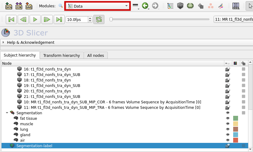
The labelmap can now be found in the "Data" section.

To save the labelmap and the corresponding volume or image as NRRD files, follow these steps:
- Select "Save" from the toolbar.
- Tick "Show options" as shown in the graphic below.
- Choose "NRRD (.nrrd)" as file format.
- Do not tick "Compress" because nnU-Net needs uncompressed data.
- For our segmentation we used the volume 7 t1_fl3d_nonfs_tra_dyn, so we save this file in the imagesTr directory and the segmentation file in the labelsTr directory.
- Save.

Change the file names
The names of the training images (in the imagesTr directory) should include the description, an ID (three digit integer) and the channel or modality (four digit integer). The modality is the type of images, for example if your dataset contains MRI and ultrasound images, the MRI images could be the modality 0000 and the ultrasound images the modality 0001. Here are some examples:
The names of the corresponding segmentation files (in the labelsTr directory) should include the description and the image ID, to which the segmentation is associated:
Mount Drive
After we generated the required directories and uploaded our data to Google Drive, we have to mount Drive in Google Colab by using the following code in a new code cell:
from google.colab import drive
drive.mount('/content/drive', force_remount = True)
A popup window will appear, where you have to connect to your Google account. After that, you should be able to access your data in Colab.
Generate a JSON file
To save some meta data reguarding the dataset, a JSON file has to be generated. We can do this automatically by using the generate_dataset_json() function from the nn-Unet package.
from nnunetv2.dataset_conversion.generate_dataset_json import generate_dataset_json

generate_dataset_json('./nnUnet_raw/Dataset011_Breast', # insert the right path to the dataset directory
                        channel_names = {0: 'MRI'},
                        labels = {
                            'background': 0,
                            'fat tissue': 1,
                            'muscle': 2,
                            'lung': 3,
                            'gland': 4,
                            'air': 5
                        },
                        num_training_cases = 5, # amount of training cases
                        file_ending = '.nrrd')
The JSON file for example contains the names of the labels and which integer values are corresponding to what label. It also contains the number of training cases, so it can later be checked if this amount of training cases are really included in the dataset folder. For this example, the file should look like this:
{
    "channel_names": {
        "0": "MRI"
    },
    "labels": {
        "background": 0,
        "fat tissue": 1,
        "muscle": 2,
        "lung": 3,
        "gland": 4,
        "air": 5
    },
    "numTraining": 5,
    "file_ending": ".nrrd"
}
Your dataset directory should now be structured as shown in the following graphic.
Set environment variables
To make sure, that nnU-Net can locate the directories of your datasets, you have to set environment variables in your system. For this, create a new code block in your notebook and run the following code.
import os

os.environ['nnUNet_raw'] = "/content/drive/MyDrive/ColabNotebooks/nnUNet/nnUNet_raw"
os.environ['nnUNet_preprocessed'] = "/content/drive/MyDrive/ColabNotebooks/nnUNet/nnUNet_preprocessed"
os.environ['nnUNet_results'] = "/content/drive/MyDrive/ColabNotebooks/nnUNet/nnUNet_results"
Be aware, that you have to choose the right path to the respective directory.
To test, if the environment variables are correctly set, you can also use the command !echo ${nnUNet_raw} afterwards. If the right path of your nnUnet_raw directory is shown as output, you can go on to the next step of the tutorial. If the output is empty, you should check if you spelled everything right and try again.
Preprocess data
Before we can train the model with our images, the dataset has to be preprocessed. To do this, we can execute the following command:
!nnUNetv2_plan_and_preprocess -d 011 --verify_dataset_integrity
The dataset ID 011 has to be exchanged for the right ID of your dataset, that you want to use.
After preprocessing, a new directory including a preprocessed version of your dataset should appear in the nnUNet_preprocessed directory.
Train model
To train the model, we also just have to use one single command:
!nnUNetv2_train 011 3d_lowres 1 -tr nnUNetTrainer_5epochs
Here are some of the options, that can be chosen from:
011is again the ID of the used dataset.- We choose
3d_lowresbecause we have 3D images with a low resolution. There are also the options3d_fullres,2dand3d_cascade_lowres. - The default number of training epochs is 1000. Because it would take a long time to train with this setting, we add
-tr nnUNetTrainer_5epochsto only train for 5 epochs. To check, which numbers of epochs you can use whithout programming an own class, click here. - As device it is recommended to use a powerful GPU, but if your computer doesn't have one (and if you don't use Colab), you can add
-device cputo execute the training on the CPU.
In most cases, the training will take one to a few hours (depends on the amount of epochs). If you want to interrupt it, click on "Interrupt execution" and use the following command the next time, you want to continue the training.
!nnUNetv2_train 011 3d_lowres 1 -tr nnUNetTrainer_5epochs --c
While the model is being fitted, you will get an output after each epoch, which will include some information like the training loss and validation loss and how long an epoch takes:

Test model
Now, that we have a trained model, we can test it by letting it predict the segmentation of a 3D volume, which wasn't part of the training data. Use the following code:
!nnUNetv2_predict   -i /content/drive/MyDrive/ColabNotebooks/nnUNet/nnUNet_raw/Dataset011_Breast/imagesTs
                    -o /content/drive/MyDrive/ColabNotebooks/nnUNet/nnUNet_raw/Dataset011_Breast/imagesTs/predictions
                    -d 011 -tr nnUNetTrainer_5epochs -c 3d_lowres -f 1
The configurations we used are listed below.
- With
-ifollowed by a path you can choose the input folder, where your test images are saved. -ochooses the output folder, where the predicted segmentations should be saved (if the directory doesn't exist, it will be automatically created).-d 011 -tr nnUNetTrainer_5epochs -c 3d_lowresmeans, that we want to choose the model, that was trained for 5 epochs with the dataset 011, including 3D low resolution images.-f 1is used to choose, with which fold of the cross validation the model was trained.
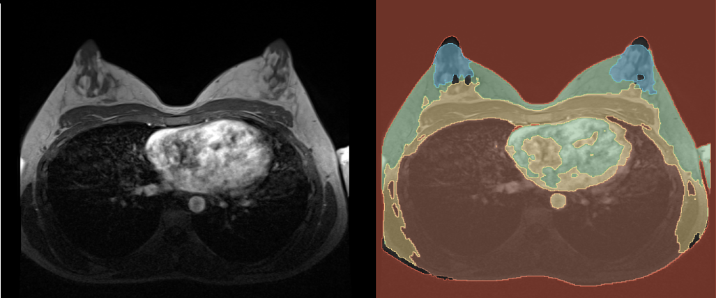
After the prediction is done, you can find the predicted segmentation in the chosen output folder. You can open it in 3D Slicer along with the reference volume to see how it turned out. In the following graphic you can see our example. You probably get a better result, if you train the model with more images and for more epochs, but also the time, the training takes, will be longer.

References
-
Isensee, F., Jaeger, P. F., Kohl, S. A., Petersen, J., & Maier-Hein, K. H. (2021). nnU-Net: a self-configuring method for deep learning-based biomedical image segmentation. Nature methods, 18(2), 203-211.
-
https://github.com/MIC-DKFZ/nnUNet/blob/master/documentation/set_environment_variables.md
-
https://github.com/MIC-DKFZ/nnUNet/blob/master/documentation/how_to_use_nnunet.md
-
https://github.com/MIC-DKFZ/nnUNet/blob/master/documentation/dataset_format.md
-
https://github.com/MIC-DKFZ/nnUNet/blob/master/nnunetv2/dataset_conversion/generate_dataset_json.py